Introduction to Material Calibration App

The Structural Roles on the 3DEXPERIENCE Platform make use of the Abaqus solver. It has many Mathematical Material Models with the help of which, we can simulate the behavior of different types of Engineering Materials like Metallic Alloys, Elastomers, Composites, and Polymer Foams under different loading conditions.

These Material Models consist of a Mathematical Equation which describes the constitutive behavior of a Material. This equation consists of parameters that the user needs to define when setting up an analysis.

For example, the below Mooney Rivlin Model typically used to model hyperelastic behavior in elastomers is

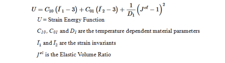
To use this model the user needs to specify the values of C10 , C01 and D1 as an input, which depend on the elastomer material. However, in many cases an Engineer only receives Experimental test data of the Material and must find out these material parameters (C10 , C01 and D1 ) and ensure that the material model curve fits accurately with the test data curve, to use a particular material model.

This is where the Material Calibration Application on the 3DEXPERIENCE Platform can be helpful. The application makes use of various Curve Fitting Algorithms with the help of which we can find out the optimized material parameters which give the best fit of the material model curve plot with the test data curve.

Let’s take a deep dive into the Material Calibration App and its functionalities. We will go through this with the help of an example, where we will run a material calibration analysis to find the optimized material parameters for a material model, with the help of a given test data.

Importing Test Data

We begin with an Experimental test data of a Rubber sample which has been tested by performing a Uniaxial Tension test, an Equibiaxial Tension test, a Planar Tension test and a Volumetric Test. The Stress vs Strain data of all the 4 tests can be imported into the Material Calibration App.

Test data is often obtained in raw form after an experiment. The data points may not start at (0,0) due to slack during experimental testing, it may even have repeated rows of same data or even noise in the data.

Using the “Zero Shift” feature we can ensure that the stress vs strain test data coincides with the origin. The “Repair” feature helps to remove repeated test data points and also ensure a monotonically increasing Nominal stress vs Nominal strain curve. Noise in the test data (due to improper specimen set up or improper load cell selection) can be removed out using the “smooth” feature which uses the Savitzky-Golay digital Filter. “Decimate” feature can be used to reduce the number of test points while still maintaining the original shape of the test data curve. Too many test points can slow down the calibration analysis.

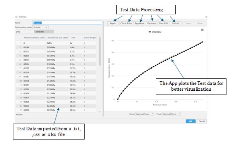
Fig 1

The Experimental Test data can be imported as a True or Nominal, Stress vs Strain data points. We can even specify the strain rate of the experimentation to include rate dependent behaviour. However, the app always plots the test data as a Nominal Stress vs Nominal strain curve.

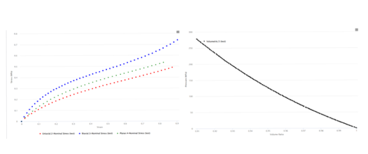
Fig 2

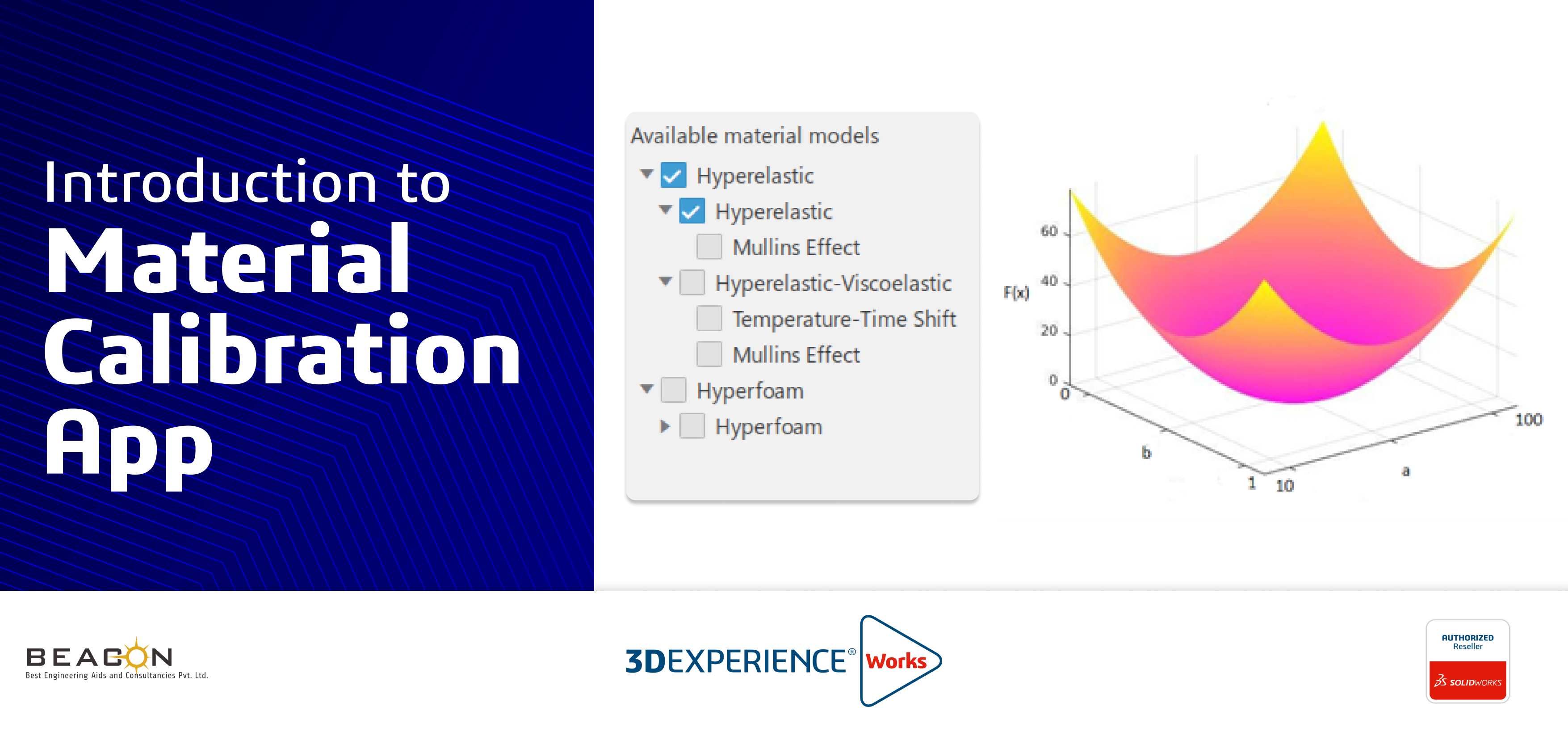
The Test Data of all the 4 experiments are plotted in the app once the data is imported, as shown in Fig.2. We then select the Material Behaviour, which we know our Test Material would exhibit, under the Physical Loading Conditions, as seen in Fig.3. As we have imported Volumetric test data also, the app gives us the options to select either the Hyperelastic or Viscoelastic Behaviour or a combination of both. We can even model the Damage Behaviour using Mullins’ Effect.

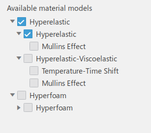
Fig 3

In this case we select the Hyperelastic Behaviour only. After that we need to select the Hyperelastic Material Model we want to calibrate, as seen in Fig.4. Here, we go with the Ogden (3rd order) Model, as we have the test data for the complete Mechanical Behaviour i.e. Uniaxial, Compression, Shear and Volumetric. There are many other Hyperelastic Models available like Neo-Hookean, Polynomial, Mooney Rivlin, Yeoh, Marlow and Polynomial.

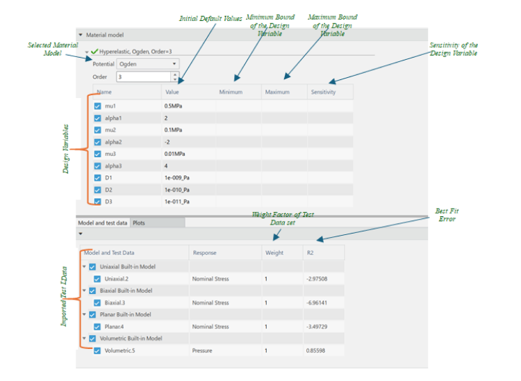
Fig 4

Fig.4 shows the Calibration Set-up dialog box, once we have selected the Material Model. The Ogden Model Parameters μ1,α1, μ2, α2, μ3, α3, D1, D2 and D3 are our Design Variables, whose optimum values need to be found out. The app has taken Default Initial Values for these parameters before running the calibration analysis as seen in fig.4.

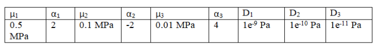
Table 1 : Initial Default Value of the Design

The bottom half of the Calibration set-up dialog box consists of the Test data rows. The 4 Test data sets i.e. Uniaxial, Biaxial, Planar and Volumetric are seen in fig.4. Each test data set has its Weight and Best Fit Error Measure value. We can assign a Weight Factor (Wi) to each data set.

The Best Fit Error Measure value shows the quality of fit between the Test Data and the projected behavior of the Material model with the help of an Error or a Deviation Value. In Fig.4 the R2 (Coefficient of Determination) value is kept as the error measure. Closer is the value of R2 to 1, better will be the fit of the Material Model Response Curve with the Test Data Curve. We can even set, either the Mean Square Error(MSE), Mean Absolute Error(MAE), Root Mean Square Error(RMSE) or the Relative Square Error (RSE) as the parameter for Best Fit Error Measure.

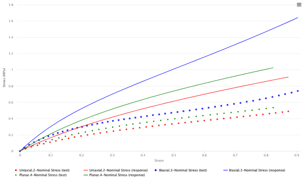
Fig 5

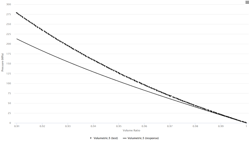
Fig 6

Fig.5 and Fig.6 show the plot of the Test data (dotted line) and the Initial Response plot (Solid Line) of the Material Model based on the Default Initial values of the Design Variables for the Ogden Model. The Response plot does not fit well with the Test Data plot initially, before running the calibration. Even the R2 values of each test data is not close enough to one (Fig.4).

Working of the Application

How Does the Material Calibration app find the optimized values of the Design Variables? It makes use of Algorithms developed for Minimizing an Objective Function.

Let’s look at this with the help of an example. If we have a Material Model, with say two Model Parameters ‘a’ and ‘b’. Therefore, ‘a’ and ‘b’ are our Design Variables whose optimum values need to be found out, such that the response plot of the Material Model fits well with the Test Data plot.

Also ‘a’ can take values between 10 and 500 and ‘b’ can take values between 0 and 1.
Now suppose, we have two test data set available for the material, one test data set for uniaxial tension and the other for uniaxial compression.

Therefore,

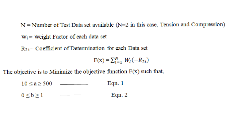
Equation 1 and 2 are our Constraint Equations.

For the Design Variable ‘a’, 10 is the Minimum Bound and 500 is the Maximum Bound on that variable. For the Design Variable ‘b’, 0 is the Minimum Bound and 1 is the Maximum Bound on that variable. Therefore, a and b would define the Design Space in which the algorithm tries to find out the optimum solution as seen in Fig.7.

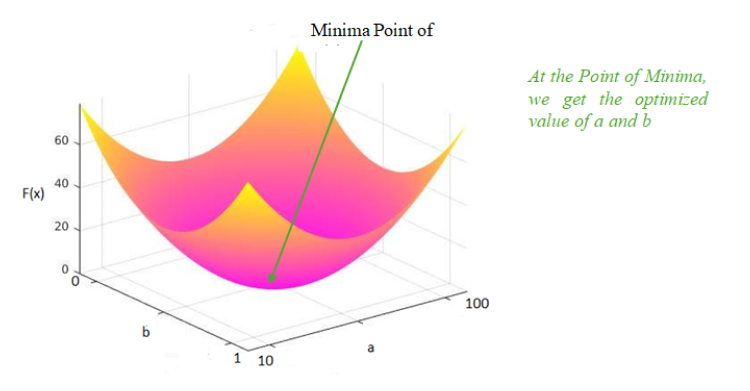
Fig 7

These minimum and maximum bounds for each design variable can be filled in the tabs in Fig.4 manually. Also, based on the Material Model being used, in many cases the app inherently defines the minimum and maximum bound on a variable automatically. For e.g. the bound for the Prony series term gi in the viscoelastic material model is between 0 and 1, hence this would be defined automatically by the app and the user need not define it.

To find the Minima point of the Objective Function the app makes use of either of the Algorithms, listed in Table 2 below.

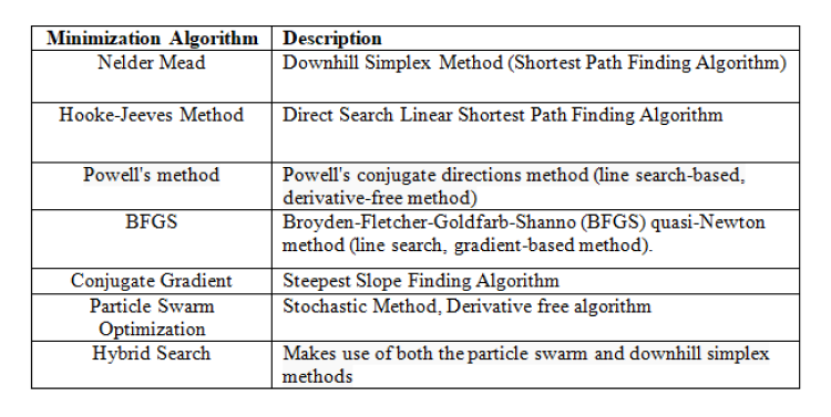
Table 2: Algorithms available in the Material

The Algorithm to be used needs to be selected by the user in the Optimization Control Settings. The Particle Swarm Optimization and Hybrid Search are the most Advanced algorithms, which can find the optimized value even for a large number of Design variable problem.

They have an advantage over the other algorithms i.e. they explore the entire design space and will always give the optimized solution at the Global Mimima of the Design space unlike the other path finding and steepest descent algorithms which may give false convergence at a Local Minima of the design space when there are many design variables.

Hence, it is recommended to run a calibration analysis with the Particle Swarm Optimization first which would give an optimized result near the global minima, and then run a second analysis using results of the first one, with the help of any of the path finding or steepest slope finding algorithm, to fine tune the results.

Running the Material Calibration Analysis

Once the Test data is imported and the Material Model to be calibrated is selected, we set up the optimization controls settings by selecting the Algorithm to be used. In this case we use the Nelder-Mead Algorithm and set up the Tolerance and Maximum number of Iterations to be done as seen in Fig.8.
We then run the Calibration Analysis. After the Analysis is completed the updated values of the Design Variables, which are optimized are shown in the Table (Fig.9).

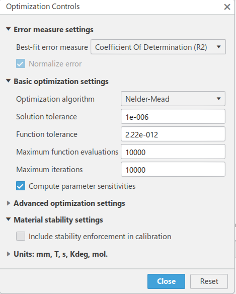
Fig 8: Optimization Control Settings

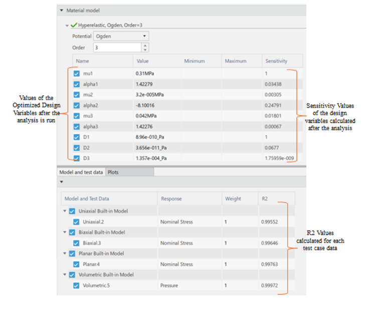
Fig 9

In Fig.9 we can also see that the App has calculated the Normalised Sensitivity value of each design variable. Variables having lower sensitivity value (near to zero) has less influence on the Objective Function. Variables with Sensitivity value near to one have high influence on the Objective Function.

We can even run a second calibration analysis, using another algorithm which uses the current calculated values of the Design variables as the Initial Values for the next calibration. Design Variables which are less sensitive can also be excluded from this analysis. This is done to further optimize the Design Variables to get a much better Fit.

In Fig.9 we can also see the new calculated value of R2 for each test data case, which is now near to one, which means that the error between the Material response plot and the test data plot is reduced.

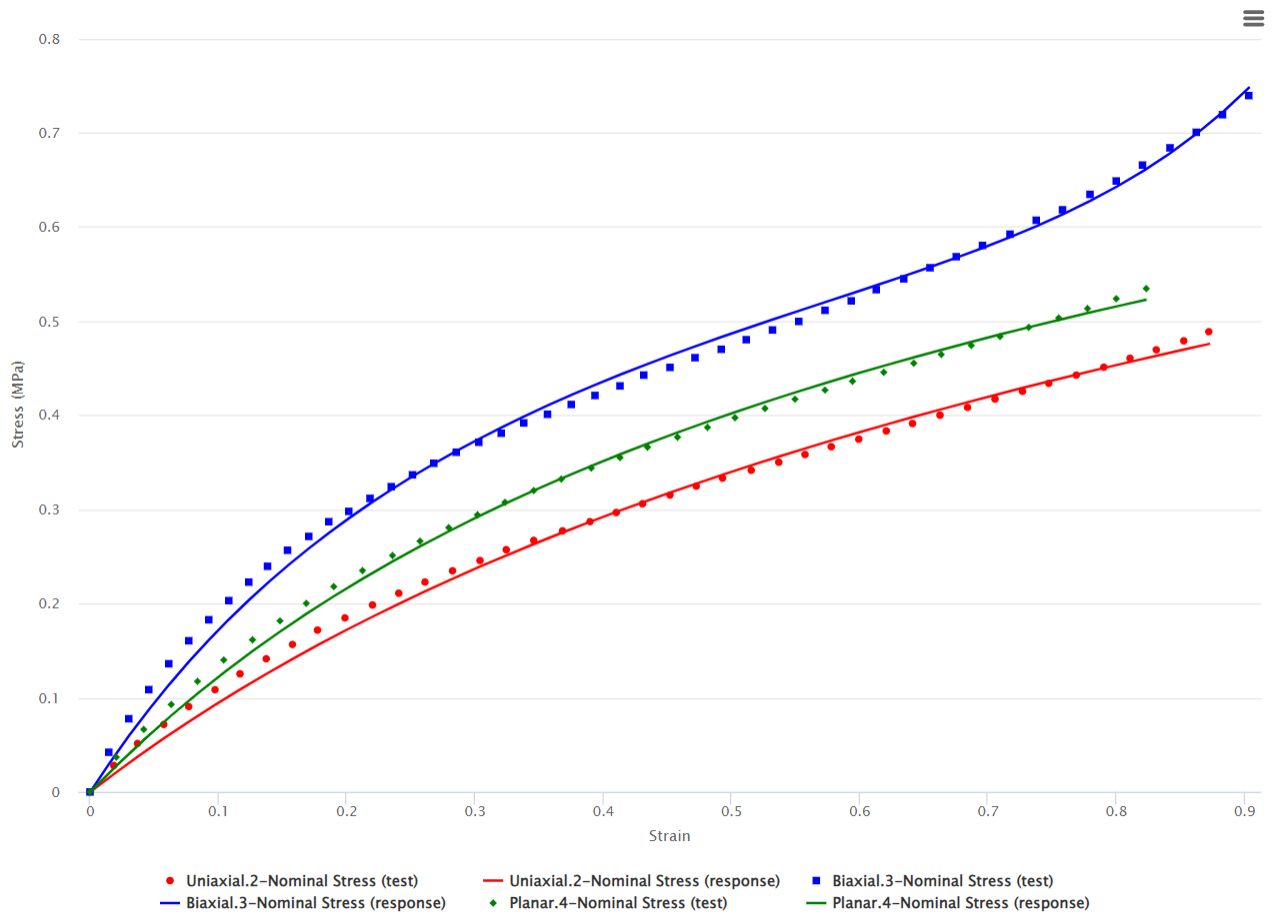
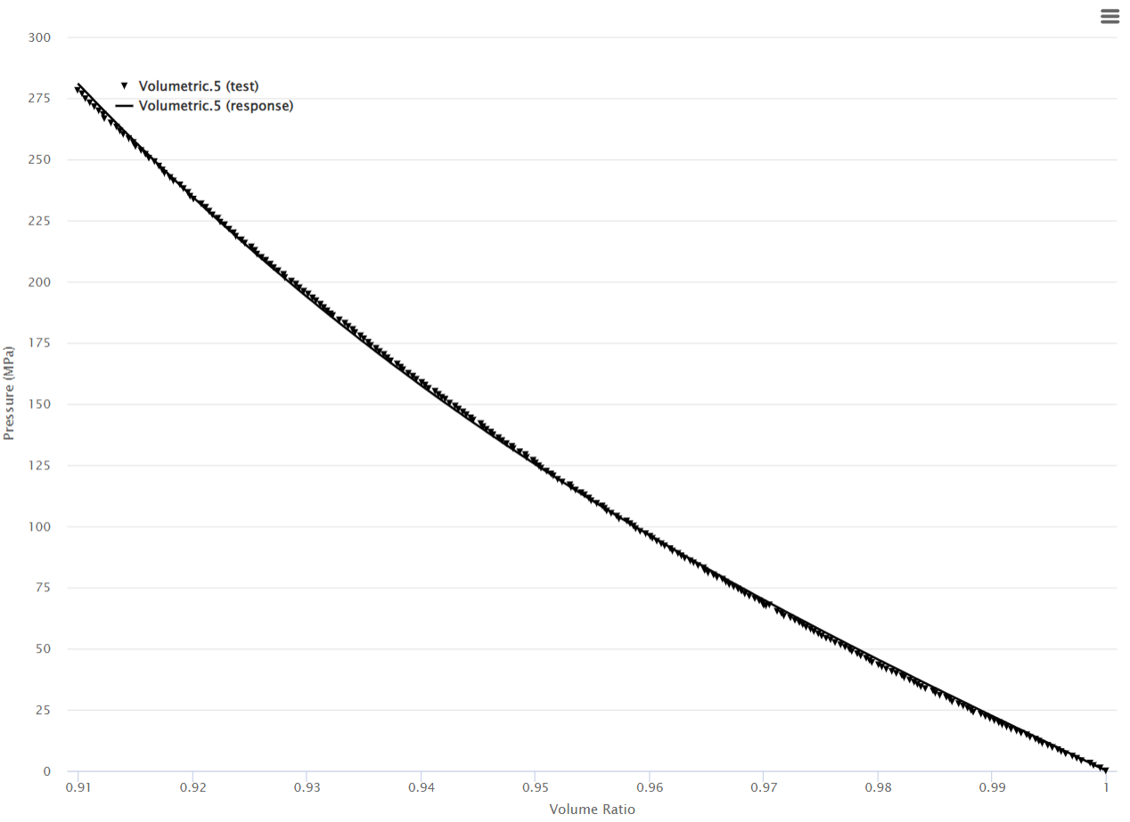
Fig 10

The Material Model Response plot fits very well with the test data plot after the calibration analysis as seen in Fig.10.

Stability of the Material

For Hyperelastic Elastic Materials we can also check the Drucker stability of the Material. The success of a Finite Element Analysis of the rubber material, which was calibrated by us, depends on the Material Model Stability.

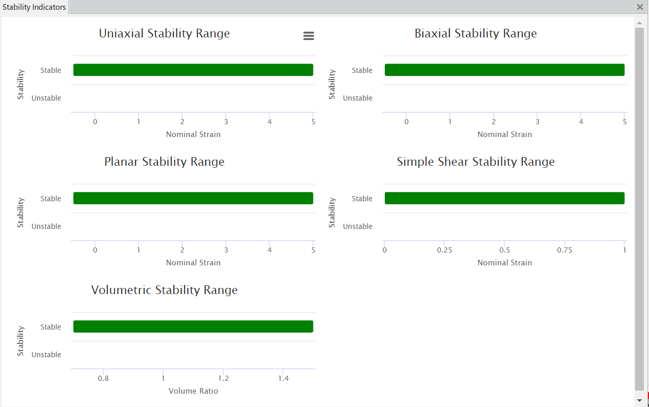
Fig 11

The Stability range of the Rubber material is shown in Fig.11 for different load cases. The Strain ranges for which the Material will be stable is highlighted in green. It is therefore recommended that the strains during a Finite element analysis should also be in this range only, to get accurate and converged results.

Lastly, we can also save the calibrated material parameters (Design Variables) in the form of a material data, which can then be used during a finite element analysis.

We Urge You To Call Us For Any Doubts & Clarifications That You May Have. We Are Eager to Talk To You

Call Us: +91 7406663589