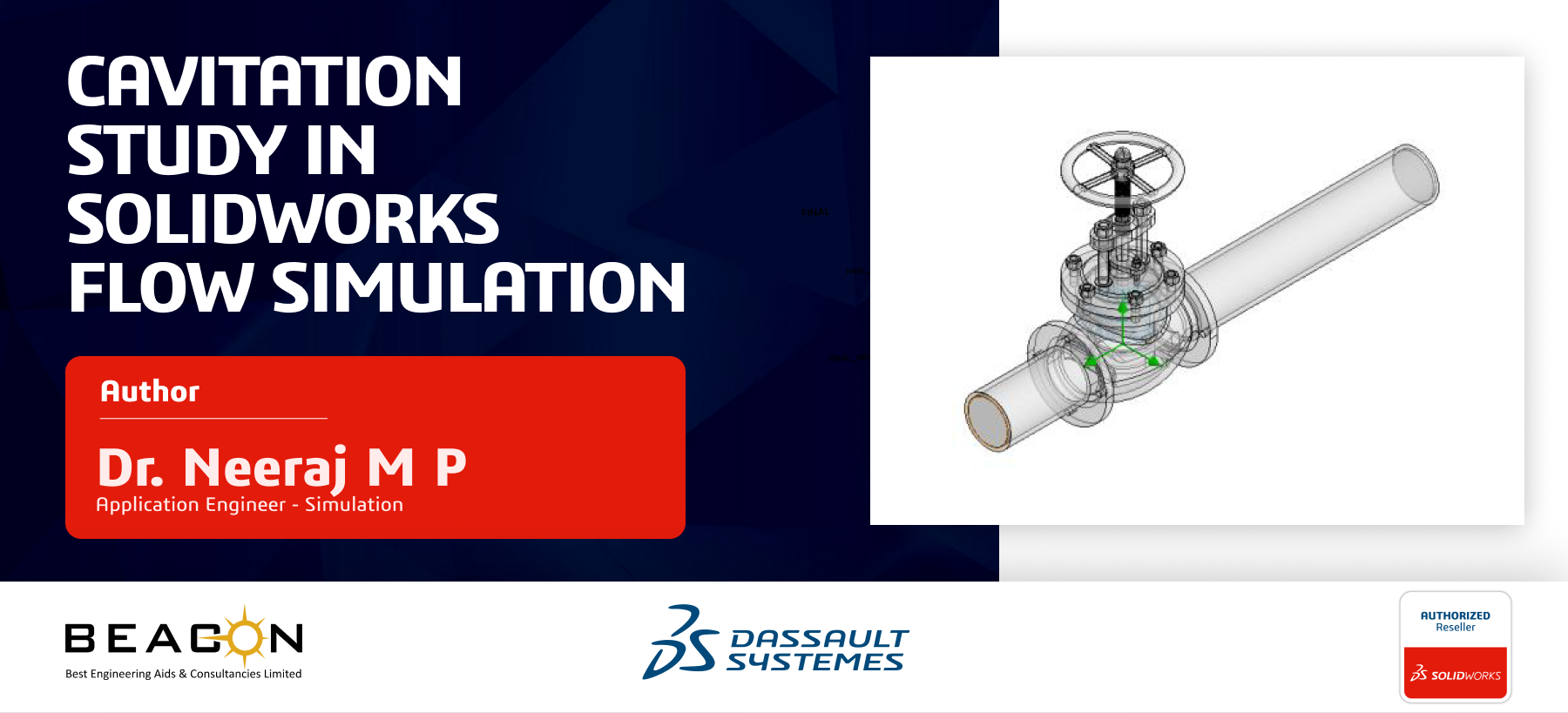
CAVITATION STUDY IN SOLIDWORKS FLOW SIMULATION

Cavitation occurs when the local pressure in a liquid fall below the saturation pressure at the local temperature. The liquid then undergoes a phase transition and vapor-filled cavities form. In hydraulic components, this commonly occurs near restrictions where the flow accelerates, and static pressure reaches a local minimum.
The SOLIDWORKS Flow Simulation has Equilibrium Cavitation Model for predefined Water and an Isothermal Cavitation Model for user-defined liquids. Both treat the cavitating medium as a homogeneous two-phase mixture at the engineering continuum level.

Equilibrium model

ρ = 1 / ν
ν = yᵍ Rᵤₙᵢᵥ T / (P μᵍ) + (1 − yᵍ − yᵥ) νₗ(T, P) + yᵥ [Rᵤₙᵢᵥ T zᵥ (T, P) / (P μᵥ)]

where ν is the specific volume of the gas-liquid mixture, νₗ is the specific volume of liquid, zᵥ(T, P) is the vapor compressibility ratio, Rᵤₙᵢᵥ is the universal gas constant, P is the local static pressure, T is the local temperature, yᵥ is the mass fraction of vapor, μᵥ is the molar mass of vapor, yᵍ is the mass fraction of the non-condensable gas; μᵍ is the molar mass of the non-condensable gas.

The properties of the dissolved non-condensable gas are set to be equal to those of air. By default, the mass fraction of non-condensable gas is set to 10-4. This is a typical model value appropriated in most cases but it can be modified by the user in the range of 10-3…10-5.
The mass fraction of vapor yᵥ is computed numerically from the following non-linear equation for the full enthalpy gas-liquid mixture:

H = yᵍ hᵍ(T, P) + (1 − yᵍ − yᵥ) hₗ(T, P) + yᵥ hᵥ(T, P) + Iᶜ yᵥ² / 2 + k / 2

where temperature of the mixture T is a function of pressure P and yᵥ. Here hg, hl, hv are the enthalpies of non-condensable gas, liquid and vapor, respectively, k is the turbulent energy, Ic is the squared impulse defined as:

Iᶜ = (ρuₓ)² + (ρuᵧ)² + (ρu_z)²

Isothermal cavitation model

The Isothermal Cavitation Model assumes that the process is approximately isothermal and that the two-phase mixture follows a barotropic pressure–density relation. The Technical Reference describes a two-phase transition between a vapor-dominated region and a compressible-liquid region.

ρ = [(P − Pᴱ(T₀)) / (Rᵤₙᵢᵥ T₀)] · (μᵍ / yᵍ), Pᴱⱽ ≤ P ≤ Pᴱᴸ

where Rᵤₙᵢᵥ is the universal gas constant, P is the local static pressure, T₀ is the local temperature, Pᴱ is the saturation pressure of liquid at T0, is the local static pressure at which the vapor appears, is the local static pressure at which the liquid turns into the vapor completely, yᵍ is the mass fraction of the non-condensable gas; μᵍ is the molar mass of the non-condensable gas.

When the pressure is below Pᴱⱽ, a liquid disappears from the mixture, and the fluid is treated as an ideal gas with the molar mass μ0. In this case the density of the gas mixture is calculated as:

ρ = P / (Rᵤₙᵢᵥ T₀) · [ yᵍ/μᵍ + (1 − yᵍ)/μ₀]⁻¹, P ≤ Pᴱⱽ

When the pressure is above the saturation pressure Pᴱᴸ, the fluid density equals the compressible liquid density

ρ = ρᴱᴸ + (P − Pᴱᴸ) / a², P ≥ Pᴱᴸ

For the Isothermal model, the dissolved-gas mass fraction is variable, and the available dissolved gases are Air, Carbon dioxide, Helium and Methane. The required liquid data include density, molar mass, saturation pressure and dynamic viscosity at the reference temperature.

Cavitation in a Globe Valve

The supplied globe-valve results demonstrate how geometry, density and vapor mass fraction should be interpreted together. The plug/seat restriction creates the accelerated flow region in which the local pressure can become sufficiently low for vapor formation.

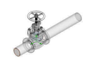
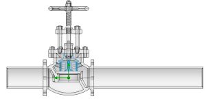
Figure 1. Globe-valve geometry and sectional view showing the plug, seat and restricted flow passage.

For this 2.5” valve standard inlet and outlet lengths (according to test standards 2D and 6D where D is the diameter) are used. Initial dissolved gas mass fraction is given as 0.002. Default The inlet flow rate is 0.028 m3/s (100 m3/hr) and outlet is exposed to environmental pressure. Local mesh refinement is used at the center where flow opening is critical. Engineering surface goals are created for pressure at inlet and outlet, and pressure drop is generated as equation goals. These goals are used for convergence mapping. The results are obtained after calculation which are shown below. The density variation and vapor mass fraction distribution can be visualized from the results.

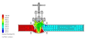
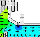
Figure 2. Fluid-density contour through the globe valve (zoomed in image shows lower density side where vapor will form)

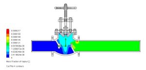
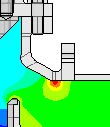
Figure 3. Vapor mass fraction contour (the red zone shows the exact vapor generation/cavitation zone)

The density field changes strongly through the valve passage and downstream region. The velocity vectors are also shown which indicates the flow direction. In a cavitating calculation, this change is associated with the altered composition of the gas–liquid mixture. Density is therefore a useful supporting result, while vapor mass fraction gives a more direct indication of predicted vapor content. The non-zero vapor-mass-fraction region is concentrated around the valve passage and extends into the downstream flow. This indicates predicted vapor content under the simulated operating condition.

Conclusion

The SOLIDWORKS Flow Simulation cavitation model provides an effective engineering approach for identifying and evaluating regions where liquid–vapor phase change is predicted. For the globe valve studied, the results demonstrate that the restricted plug-and-seat passage creates the conditions for vapor formation, with the predicted vapor region concentrated around the high-velocity flow passage and extending downstream. The combination of pressure, density, and vapor mass fraction provides a more complete understanding of the cavitation behavior than any single contour alone.

We Urge You To Call Us For Any Doubts & Clarifications That You May Have. We Are Eager to Talk To You

Call Us: +91 7406663589